Quick Start

Colab Notebook (Recommended)

For the fastest start, run the full workflow notebook in Google Colab:

• Open in Colab

• Notebook source on GitHub

This notebook includes package installation, Google Drive setup, preprocessing, runoff/routing, training, evaluation, and simulation in one guided flow.

1) Setup working directory and study area

Define where all intermediate and output files will be stored, and the basin boundary shapefile that defines the spatial extent of the workflow. The shapefile should be in EPSG:4326 (WGS84) so that all raster downloads and clipping steps align correctly.

At this stage you are only defining paths; no files are created yet. All subsequent modules will read from and write to subfolders under working_dir. Keep the basin shapefile small and clean (single polygon) to avoid clipping issues.

Expected outputs:

• Folders under working_dir created by later steps (e.g., elevation/, soil/, ndvi/, vcf/).

Common pitfalls:

• Shapefile in a different CRS (reproject to EPSG:4326).

• Shapefile path points to the wrong basin or an empty geometry.

working_dir = "/path/to/working_dir"
study_area = "/path/to/basin.shp"

2) Download and preprocess input data

These steps download and prepare static inputs (vegetation, DEM, soil, AlphaEarth) and dynamic forcing (meteorology). Most inputs are clipped to the study area and saved under working_dir for later stages.

Run these once per basin. If you change the basin boundary or the DEM resolution, re-run the preprocessing steps so all inputs align. For Earth Engine-based datasets, the first run will prompt for authentication.

Recommended preprocessing order:

• DEM first, then Tree cover, NDVI, Soil, AlphaEarth, and Meteorology.

• DEM creates the reference grid (elevation/dem_clipped.tif) used to align the other raster inputs.

Dataset availability windows:

• Tree cover (MODIS VCF): available from 2001 onward.

• NDVI (MODIS 16-day): available from 2001 onward.

• AlphaEarth embeddings: available from 2017 onward.

Google Earth Engine authentication

Several inputs (NDVI, Tree cover, AlphaEarth, and ERA5/CHIRPS via Earth Engine) require Google Earth Engine (GEE). The first time you run these modules, you will be prompted to authenticate.

Typical workflow:

• Register for a GEE account in the Earth Engine Code Editor. Code Editor: https://code.earthengine.google.com/

• The Earth Engine Python API is installed as part of the project dependencies.

• Run any module that calls ee.Authenticate() (e.g., NDVI or TreeCover).

• A browser window will open with a Google login prompt.

• After login, copy the authorization code back to the terminal.

If you are on a headless server:

• Run earthengine authenticate on a machine with a browser.

• Copy the generated credentials (~/.config/earthengine/credentials) to the server under the same path.

Expected outputs:

• Raster files in ndvi/, vcf/, elevation/, soil/, alpha_earth/.

• NetCDF climate files in {data_source}/.

Common pitfalls:

• Missing Earth Engine authentication (NDVI/Tree cover/AlphaEarth).

• Incomplete downloads (rerun the step).

DEM

Preprocessing and model use:

• Run this step first.

• Downloads a DEM (default 1 km), clips to the basin, and reprojects to match the project grid.

• Derives slope, flow direction, accumulation, and the river grid used for runoff routing and catchment geometry.

from bakaano.dem import DEM
dd = DEM(
    working_dir=working_dir,
    study_area=study_area,
    local_data=False,
    local_data_path=None,
)
dd.get_dem_data()
dd.plot_dem()

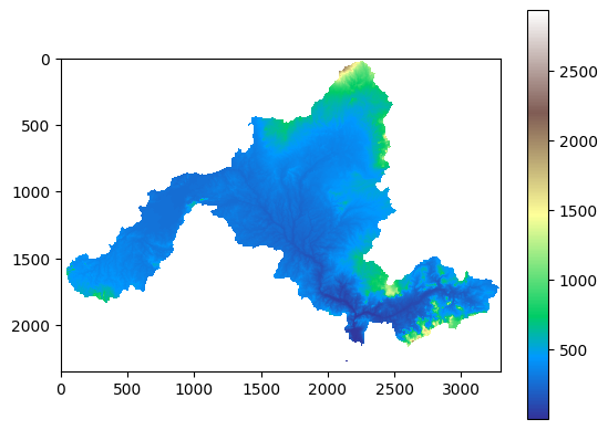
Example output: clipped DEM.

Tree cover (MODIS VCF)

Preprocessing and model use:

• Downloads annual MODIS VCF tree cover, clips to the study area, and resamples to the DEM grid so it aligns with all other rasters.

• Produces a static vegetation cover layer used by VegET and the streamflow model as a land-surface predictor.

• Source data availability starts in 2001.

from bakaano.tree_cover import TreeCover
vf = TreeCover(
    working_dir=working_dir,
    study_area=study_area,
    start_date="2001-01-01",
    end_date="2020-12-31",
)
vf.get_tree_cover_data()
vf.plot_tree_cover(variable="tree_cover")

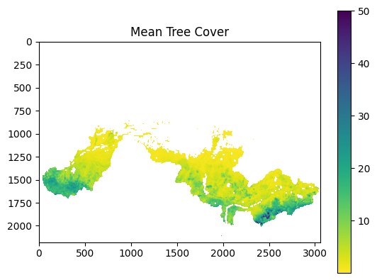
Example output: mean tree cover raster.

NDVI (MODIS 16-day)

Preprocessing and model use:

• Downloads 16-day NDVI composites, clips to the basin, and resamples to the DEM grid.

• Aggregates to climatology or interval stacks (as stored under ndvi/) used by VegET to represent vegetation dynamics and seasonal water use.

• Source data availability starts in 2001.

from bakaano.ndvi import NDVI
nd = NDVI(
    working_dir=working_dir,
    study_area=study_area,
    start_date="2001-01-01",
    end_date="2010-12-31",
)
nd.get_ndvi_data()
nd.plot_ndvi(interval_num=10)

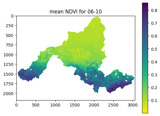
Example output: NDVI climatology for a 16-day interval.

Soil

Preprocessing and model use:

• Downloads global soil properties, clips to the basin, and resamples to the DEM grid.

• Produces soil layers (e.g., wilting point, field capacity) used by VegET to model soil moisture storage and evapotranspiration.

from bakaano.soil import Soil
sgd = Soil(
    working_dir=working_dir,
    study_area=study_area,
)
sgd.get_soil_data()
sgd.plot_soil(variable="wilting_point")

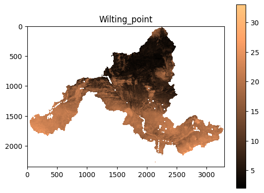
Example output: soil property raster.

AlphaEarth embeddings

Preprocessing and model use:

• Downloads AlphaEarth embedding tiles, clips to the basin, and resamples to the DEM grid.

• Stacks the embedding bands as static catchment descriptors used by the streamflow model to capture land-surface characteristics beyond basic physiography.

• Source data availability starts in 2017.

from bakaano.alpha_earth import AlphaEarth
dd = AlphaEarth(
    working_dir=working_dir,
    study_area=study_area,
    start_date="2013-01-01",
    end_date="2024-01-01",
)
dd.get_alpha_earth()
dd.plot_alpha_earth("A35")

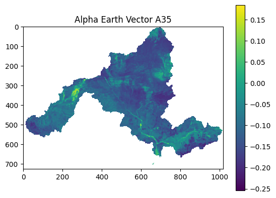
Example output: AlphaEarth band visualization.

Meteorology (ERA5 / CHIRPS / CHELSA)

Preprocessing and model use:

• Downloads meteorological variables as raster time series, clips to the basin, and resamples to the DEM grid.

• ERA5 provides the full set of variables. CHIRPS is used for precipitation only, while other variables still come from ERA5. CHELSA provides downscaled ERA5 data.

• Stores results under {data_source}/ and converts them to NetCDF stacks for efficient access during VegET runoff computation and model training.

from bakaano.meteo import Meteo
cd = Meteo(
    working_dir=working_dir,
    study_area=study_area,
    start_date="2001-01-01",
    end_date="2010-12-31",
    local_data=False,
    data_source="ERA5",
)
cd.plot_meteo(variable="tasmin", date="2006-12-01")

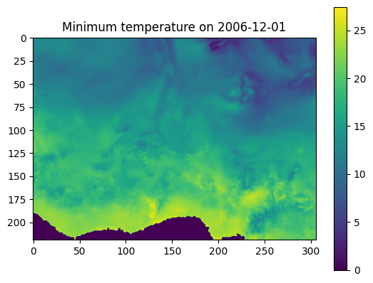
Example output: meteorological field.

3) Computing runoff and routing to river network

This step computes daily runoff using VegET and routes it to the river network. Outputs are stored in runoff_output and are used as predictors for streamflow model training and simulation.

The runoff computation depends on the DEM grid. If you provide a higher resolution DEM, the runtime will increase and outputs will be larger. Make sure you have enough disk space for the routed runoff files.

Expected outputs:

• Routed runoff pickles in runoff_output/.

• River grid in catchment/river_grid.tif (if generated).

Common pitfalls:

• DEM missing or not clipped to basin.

• Missing NDVI/tree cover/soil inputs.

• Unsupported climate_data_source value. Use "CHELSA", "ERA5", or "CHIRPS".

from bakaano.veget import VegET
vg = VegET(
    working_dir=working_dir,
    study_area=study_area,
    start_date="2001-01-01",
    end_date="2010-12-31",
    climate_data_source="ERA5",
    routing_method="mfd",
)
vg.compute_veget_runoff_route_flow()

Long runs can be resumed:

vg.compute_veget_runoff_route_flow(
    resume=True,
    checkpoint_days=30,
)

Notes:

• resume=True reuses matching checkpoint state in runoff_output/ if an earlier run was interrupted.

• checkpoint_days controls how often routed runoff chunks are flushed to disk.

• The final routed runoff product is runoff_output/wacc_sparse_arrays.pkl.

Visualize routed runoff

from bakaano.plot_runoff import RoutedRunoff
rr = RoutedRunoff(
    working_dir=working_dir,
    study_area=study_area,
)
rr.map_routed_runoff(date="2020-01-03", vmax=7)

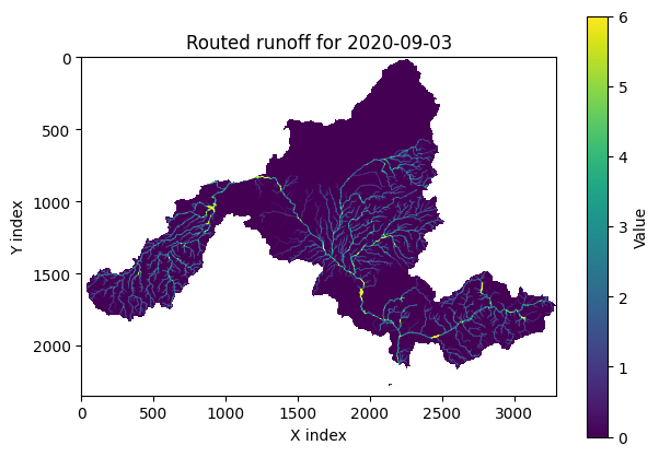
Example output: routed runoff map.

Interactive routed runoff timeseries

This opens an interactive plot that lets you explore routed runoff time series for stations in your study area. Provide GRDC NetCDF or a station lookup CSV (id + coordinates). Use it to spot missing data, unrealistic peaks, or routing artifacts before training. You will be prompted in the terminal to select a station.

# Option 1: GRDC NetCDF stations
rr.interactive_plot_routed_runoff_timeseries(
    start_date="2000-01-01",
    end_date="2000-12-31",
    grdc_netcdf="/path/to/GRDC.nc",
)

# Option 2: Station lookup CSV (id + coordinates)
rr.interactive_plot_routed_runoff_timeseries(
    start_date="2000-01-01",
    end_date="2000-12-31",
    lookup_csv="/path/to/station_lookup.csv",
    id_col="id",
    lat_col="latitude",
    lon_col="longitude",
)

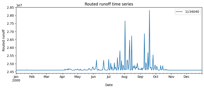
Example output: routed runoff timeseries.

4) Explore input data, river networks and stations interactively

Use the interactive map to inspect DEM, slope, vegetation, routed river network, and available hydrological stations for the study area. This is useful to verify data availability before training or simulation.

Use this step to sanity-check that stations fall inside the basin and that the raster layers align spatially. If no stations appear, your GRDC file likely does not cover the basin or the CRS is mismatched.

Expected outputs:

• An interactive map with layers and station points.

Common pitfalls:

• GRDC NetCDF does not cover the basin (no stations appear).

from bakaano.runner import BakaanoHydro
bk = BakaanoHydro(
    working_dir=working_dir,
    study_area=study_area,
    climate_data_source="ERA5",
)
bk.explore_data_interactively(
    "1989-01-01",
    "1989-12-31",
    "/path/to/GRDC.nc",
)

5) Training, evaluating and applying Bakaano-Hydro

This section trains a regional model, evaluates it interactively, and runs batch simulations. Training uses routed runoff predictors and observed streamflow targets.

Training can take hours depending on GPU and batch size. Evaluation is interactive and lets you choose stations to compare observed vs predicted streamflow. Simulation produces CSV files for each station or coordinate. Note: simulation outputs start after a one-year warmup period; the first 365 days are used as model context and are not written to the output CSVs.

Expected outputs:

• Trained model saved in models/.

• Predicted streamflow CSVs in predicted_streamflow_data/.

Common pitfalls:

• GRDC NetCDF missing required variables (runoff_mean, geo_x, geo_y).

• Station IDs not found in the dataset.

Initialize model

This creates the high-level Bakaano-Hydro object that manages training and simulation. It does not start any computation by itself, but it validates the working directory and establishes the study area context for later steps.

from bakaano.runner import BakaanoHydro
bk = BakaanoHydro(
    working_dir=working_dir,
    study_area=study_area,
    climate_data_source="ERA5",
)

Training

Training builds the TCN model (365-day input with an internal 180-day slice) and fits it using routed runoff predictors and observed discharge. You can train with GRDC NetCDF stations or with per-station CSV files via a lookup table. This step can take hours depending on GPU, batch size, and the number of stations.

Model overwrite/resume behavior:

• model_overwrite=True: start a fresh model run and overwrite the saved model file.

• model_overwrite=False: if {working_dir}/models/bakaano_model.keras exists, load it and continue training; otherwise start fresh.

Minimal training option (GRDC)

bk.train_streamflow_model(
    train_start="1981-01-01",
    train_end="2020-12-31",
    grdc_netcdf="/path/to/GRDC.nc",
    batch_size=32,
    num_epochs=300,
    learning_rate=0.001,
    lr_schedule="cosine",
    warmup_epochs=5,
    min_learning_rate=1e-5,
    routing_method="mfd",
    area_normalize=True,
    model_overwrite=True,
)

Minimal training option (CSV observations)

Requirements for CSV training:

• lookup_csv must include station ID and coordinates (default columns: id, latitude, longitude).

• csv_dir should contain one file per station.

• File naming follows file_pattern (default {id}.csv).

• Each station CSV must include a date column and discharge column (default: date and discharge).

See Inputs and Outputs for the full CSV schema and unit conventions.

Optional column overrides (if your headers differ): - id_col, lat_col, lon_col - date_col, discharge_col - file_pattern

bk.train_streamflow_model(
    train_start="1981-01-01",
    train_end="2020-12-31",
    grdc_netcdf=None,
    batch_size=32,
    num_epochs=300,
    learning_rate=0.001,
    lr_schedule="cosine",
    warmup_epochs=5,
    min_learning_rate=1e-5,
    routing_method="mfd",
    area_normalize=True,
    csv_dir="/path/to/observed_csvs",
    lookup_csv="/path/to/station_lookup.csv",
    id_col="id",
    lat_col="latitude",
    lon_col="longitude",
    date_col="date",
    discharge_col="discharge",
    file_pattern="{id}.csv",
    model_overwrite=True,
)

Notes: - Training saves scalers to {working_dir}/models (AlphaEarth). - Set area_normalize=False to train directly on raw m³/s instead of area-normalized depth (mm/day). - The current streamflow pipeline uses linear predictors/targets; there is no

extra sqrt or log response transform in training or inference.

Advanced training option (model configuration)

Parameter guidance (see bakaano.runner.BakaanoHydro.train_streamflow_model()):

• learning_rate: base optimizer step size; lower if training is unstable.

• loss_function: training objective (e.g., mse, huber, msle, asym_laplace_nll).

• seed: controls deterministic behavior where randomization is used.

• lr_schedule: cosine or exp_decay; set to None for fixed LR.

• warmup_epochs: warmup length before LR schedule ramps to base LR.

• min_learning_rate: minimum LR for schedules.

• routing_method: must match the runoff routing method used in VegET.

• catchment_size_threshold: filters very small catchments.

• area_normalize: toggle area normalization for predictors/response.

• model_overwrite: True for fresh training, False to resume from saved model.

Guidance: - Use loss_function="asym_laplace_nll" for asymmetric uncertainty. - With asym_laplace_nll, the model outputs 3 parameters; with other losses, it outputs 1 value. - Lower learning_rate if training is unstable.

bk.train_streamflow_model(
    train_start="1981-01-01",
    train_end="2020-12-31",
    grdc_netcdf="/path/to/GRDC.nc",
    batch_size=32,
    num_epochs=300,
    learning_rate=0.001,
    loss_function="mse",
    seed=100,
    lr_schedule="cosine",
    warmup_epochs=5,
    min_learning_rate=1e-5,
    routing_method="mfd",
    catchment_size_threshold=1,
    area_normalize=True,
    model_overwrite=False,
)

Evaluate interactively (GRDC)

This launches an interactive evaluation that prompts you to choose a station and then plots observed vs predicted discharge for the selected period. Use this to inspect model performance before running batch simulations. You will be prompted in the terminal to select a station.

model_path = f"{working_dir}/models/bakaano_model.keras"
bk.evaluate_streamflow_model_interactively(
    model_path=model_path,
    val_start="2001-01-01",
    val_end="2010-12-31",
    grdc_netcdf="/path/to/GRDC.nc",
    routing_method="mfd",
    area_normalize=True,
)

Advanced evaluation options (optional)

Required for model configuration: - routing_method must match the method used for runoff routing.

Guidance: - Use csv_dir and lookup_csv to evaluate with station CSVs. - Use the same area_normalize setting that was used when training the model.

bk.evaluate_streamflow_model_interactively(
    model_path=model_path,
    val_start="2001-01-01",
    val_end="2010-12-31",
    grdc_netcdf="/path/to/GRDC.nc",
    routing_method="mfd",
    catchment_size_threshold=1000,
    area_normalize=True,
    csv_dir=None,
    lookup_csv=None,
    id_col="id",
    lat_col="latitude",
    lon_col="longitude",
    date_col="date",
    discharge_col="discharge",
    file_pattern="{id}.csv",
)

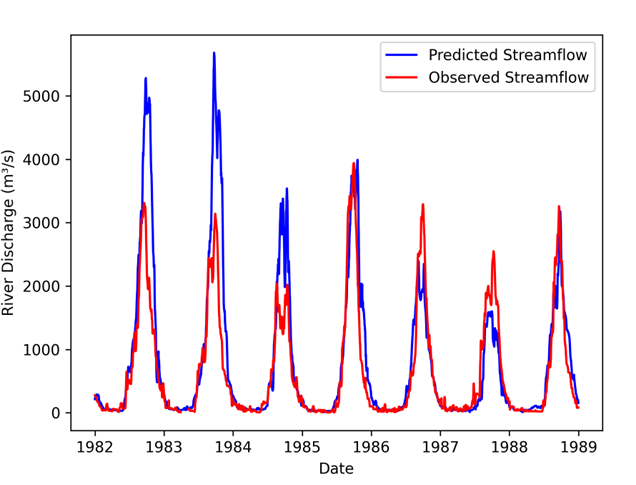
Example output: observed vs predicted streamflow from interactive evaluation.

Batch prediction for GRDC stations

This runs inference for all GRDC stations in the study area and writes one CSV per station to predicted_streamflow_data/. Outputs start after a one-year warmup period; the first 365 days of the simulation window are used as model context and are not written to the CSVs. Example: if sim_start="1981-01-01" and sim_end="2020-12-31", the first timestamp in the output CSV is 1982-01-01 (one year after the start date). Predictions are written in m³/s. If area_normalize=True, the model internally predicts area-normalized discharge and converts it back to m³/s before writing CSVs.

model_path = f"{working_dir}/models/bakaano_model.keras"
bk.simulate_grdc_csv_stations(
    model_path=model_path,
    sim_start="1981-01-01",
    sim_end="2020-12-31",
    grdc_netcdf="/path/to/GRDC.nc",
    routing_method="mfd",
    area_normalize=True,
)

Batch prediction with CSV stations

Outputs start after a one-year warmup period; the first 365 days of the simulation window are used as model context and are not written to the CSVs. Example: if sim_start="1981-01-01", the output begins at 1982-01-01.

bk.simulate_grdc_csv_stations(
    model_path=model_path,
    sim_start="1981-01-01",
    sim_end="2020-12-31",
    grdc_netcdf=None,
    routing_method="mfd",
    area_normalize=True,
    csv_dir="/path/to/observed_csvs",
    lookup_csv="/path/to/station_lookup.csv",
    id_col="id",
    lat_col="latitude",
    lon_col="longitude",
    date_col="date",
    discharge_col="discharge",
    file_pattern="{id}.csv",
)

Predict streamflow at arbitrary points

This simulates streamflow for user-defined coordinates inside the study area. Each coordinate produces a separate CSV output time series. Outputs start after a one-year warmup period; the first 365 days of the simulation window are used as model context and are not written to the CSVs. Example: if sim_start="1981-01-01" and sim_end="1990-12-31", the CSV starts at 1982-01-01 and runs through 1990-12-31.

model_path = f"{working_dir}/models/bakaano_model.keras"
bk.simulate_streamflow(
    model_path=model_path,
    sim_start="1981-01-01",
    sim_end="1990-12-31",
    latlist=[13.8, 13.9],
    lonlist=[3.0, 4.0],
    routing_method="mfd",
    area_normalize=True,
)

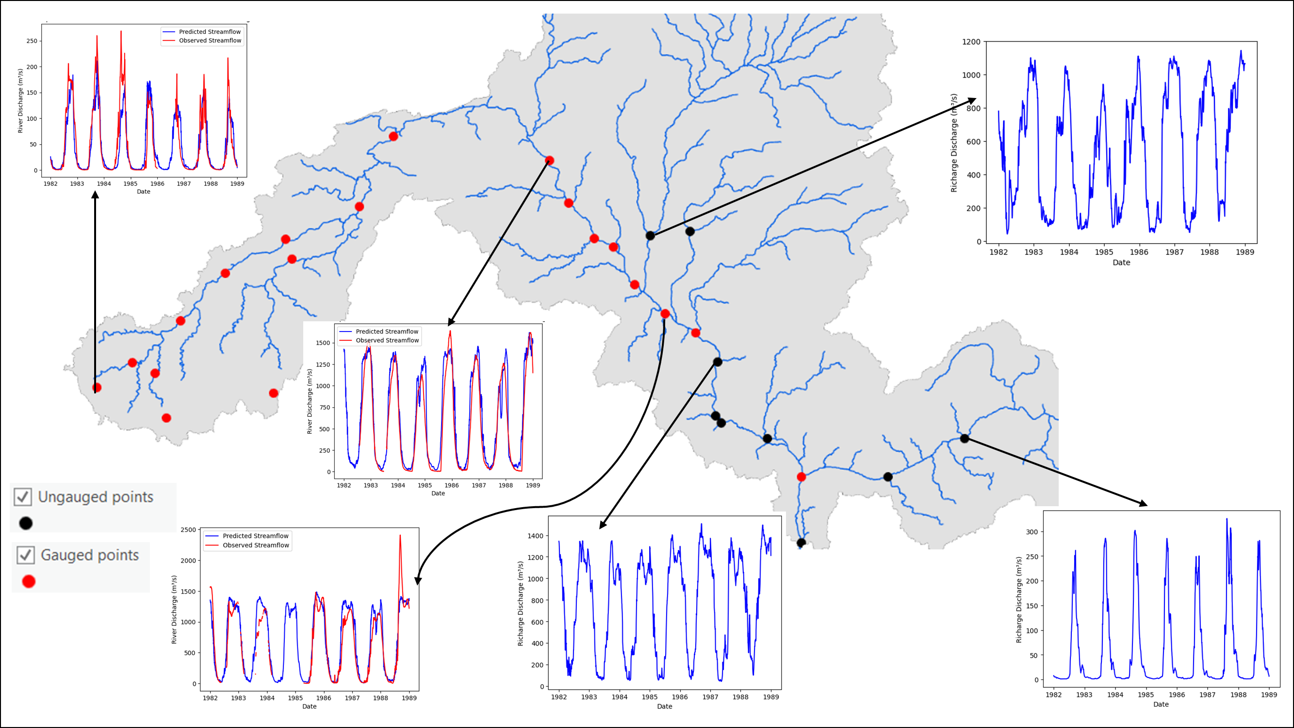
Illustration: prediction points sampled along the river network.